The variational auto-encoder

In this chapter, we are going to use various ideas that we have learned in the class in order to present a very influential recent probabilistic model called the variational autoencoder.

Variational autoencoders (VAEs) are a deep learning technique for learning latent representations. They have also been used to draw images, achieve state-of-the-art results in semi-supervised learning, as well as to interpolate between sentences.

There are many online tutorials on VAEs. Our presentation will probably be a bit more technical than the average, since our goal will be to highlight connections to ideas seen in class, as well as to show how these ideas are useful in machine learning research.

Deep generative models

Consider a directed latent-variable model of the form

with observed $x \in \mathcal{X}$, where $\mathcal{X}$ can be either continuous or discrete, as well as latent $z \in \mathbb{R}^k$.

⊕
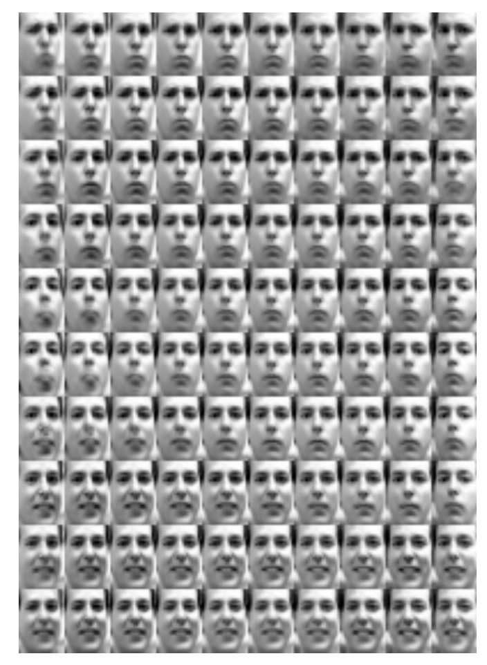
Variational autoencoder $p(x|z)p(z)$ applied to a face images (modeled by $x$). The learned latent space $z$ can be used to interpolate between facial expressions. To make things concrete, you may think of $x$ as being an image (e.g. a human face), and $z$ as being latent factors (not seen during training) that explain features of the face. For example, one coordinate of $z$ can encode whether the face is happy or sad, another one whether the face is male or female, etc.

We may also be interested in models with many layers, e.g. $p(x \mid z_1)p(z_2 \mid z_3)\cdots p(z_{m-1}\mid z_m)p(z_m)$. These are often called deep generative models and can learn hierarchies of latent representations. In this chapter, we will assume for simplicity that there is only one latent layer.

Learning deep generative models

Suppose now that we are given a dataset $D = \{x^1,x^2,...,x^n\}$. We are interested in the following inference and learning tasks:

• Learning the parameters $\theta$ of $p$.
• Approximate posterior inference over $z$: given an image $x$, what are its latent factors?
• Approximate marginal inference over $x$: given an image $x$ with missing parts, how do we fill-in these parts?

We are also going to make the following additional assumptions

• Intractability: computing the posterior probability $p(z\mid x)$ is intractable.
• Big data: the dataset $D$ is too large to fit in memory; we can only work with small, subsampled batches of $D$.

Many interesting models fall in this class; the variational auto-encoder will be one such model.

Trying out the standard approaches

We have learned several techniques in the class that could be used to solve our three tasks. Let’s try them out.

The EM algorithm can be used to learn latent-variable models. Recall, however, that performing the E step requires computing the approximate posterior $p(z\mid x)$, which we have assumed to be intractable. In the M step, we learn the $\theta$ by looking at the entire datasetNote, however, that there exists a generalization called online EM, which performs the M-step over mini-batches. , which is going to be too large to hold in memory.

To perform approximate inference, we may use mean field. Recall, however, that one step of mean field requires us to compute an expectation whose time complexity scales exponentially with the size of the Markov blanket of the target variable.

What is the size of the Markov blanket for $z$? If we assume that at least one component of $x$ depends on each component of $z$, then this introduces a V-structure into the graph of our model (the $x$, which are observed, are explaining away the differences among the $z$). Thus, we know that all the $z$ variables will depend on each other and the Markov blanket of some $z_i$ will contain all the other $z$-variables. This will make mean-field intractableThe authors refer to this when they say “the required integrals for any reasonable mean-field VB algorithm are also intractable”. They also discuss the limitations of EM and sampling methods in the introduction and the methods section. . An equivalent (and simpler) explanation is that $p$ will contain a factor $p(x_i \mid z_1,...,z_K)$, in which all the $z$ variables are tied.

Another approach would be to use sampling-based methods. In the VAE paper, the authors compare against these kinds of algorithms, but they find that they don’t scale well to large datasets. In addition, techniques such as Metropolis-Hastings require a hand-crafted proposal distribution, which might be difficult to choose.

Auto-encoding variational Bayes

We will now going to learn about Auto-encoding variational Bayes (AEVB), an algorithm that can efficiently solve our three inference and learning tasks; the variational auto-encoder will be one instantiation of this algorithm.

AEVB is based on ideas from variational inference. Recall that in variational inference, we are interested in maximizing the evidence lower bound (ELBO)

over the space of all $q_\phi$. The ELBO satisfies the equation

Since $x$ is fixed, we can define $q(z\mid x)$ to be conditioned on $x$. This means that we are effectively choosing a different $q(z)$ for every $x$, which will produce a better posterior approximation than always choosing the same $q(z)$.

How exactly do we optimize over $q(z\mid x)$? We may use mean field, but this turns out to be insufficiently accurate for our purposes. The assumption that $q$ is fully factored is too strong, and the coordinate descent optimization algorithm is too simplistic.

Black-box variational inference

The first important idea used in the AEVB algorithm is a general purpose approach for optimizing $q$ that works for large classes of $q$ (that are more complex than in mean field). We later combine this algorithm with specific choices of $q$.

This approach – called black-box variational inferenceThe term black-box variational inference was first coined by Ranganath et al., with the ideas being inspired by earlier work, such as the Wake-Sleep algorithm. – consists in maximizing the ELBO using gradient descent over $\phi$ (instead of e.g., using a coordinate descent algorithm like mean field). Hence, it only assumes that $q_\phi$ is differentiable in its parameters $\phi$.

Furthermore, instead of only doing inference, we will simultaneously perform learning via gradient descent on both $\phi$ and $\theta$ (jointly). Optimization over $\phi$ will keep ELBO tight around $\log p(x)$; optimization over $\theta$ will keep pushing the lower bound (and hence $\log p(x)$) up. This is somewhat similar to how the EM algorithm optimizes a lower bound on the marginal likelihood.

The score function gradient estimator

To perform black-box variational inference, we need to compute the gradient

Taking the expectation with respect to $q$ in closed form will often not be possible. Instead, we may take Monte Carlo estimates of the gradient by sampling from $q$. This is easy to do for the gradient of $p$: we may swap the gradient and the expectation and estimate the following expression via Monte Carlo

However, taking the gradient with respect to $q$ is more difficult. Notice that we cannot swap the gradient and the expectation, since the expectation is being taken with respect to the distribution that we are trying to differentiate!

One way to estimate this gradient is via the so-called score function estimator:

This follows from some basic algebra and calculus and takes about half a page to derive. We leave it as an exercise to the reader, but for those interested, the full derivation may found in Appendix B of this paper.

The above identity places the gradient inside the expectation, which we may now evaluate using Monte Carlo. We refer to this as the score function estimator of the gradient.

Unfortunately, the score function estimator has an important shortcoming: it has a high variance. What does this mean? Suppose you are using Monte Carlo to estimate an expectation whose mean is 1. If your samples are $0.9, 1.1, 0.96, 1.05,..$ and are close to 1, then after a few samples, you will get a good estimate of the true expectation. If on the other hand you sample zero 99 times out of 100, and you sample 100 once, the expectation is still correct, but you will have to take a very large number of samples to figure out that the true expectation is actually one. We refer to the latter case as being high variance.

This is the kind of problem we often run into with the score function estimator. In fact, its variance is so high, that we cannot use it to learn many models.

The key contribution of the VAE paper is to propose an alternative estimator that is much better behaved. This is done in two steps: we first reformulate the ELBO so that parts of it can be computed in closed form (without Monte Carlo), and then we use an alternative gradient estimator, based on the so-called reparametrization trick.

The SGVB estimator

The reformulation of the ELBO is as follows.

It is straightforward to verify that this is the same using ELBO using some algebra.

This reparametrization has a very interesting interpretation. First, think of $x$ as an observed data point. The left-hand side consists of two terms; both involve taking a sample $z \sim q(z\mid x)$, which we can interpret as a code describing $x$. We are also going to call $q$ the encoder.

In the first term, $\log p(x\mid z)$ is the log-likelihood of the observed $x$ given the code $z$ that we have sampled. This term is maximized when $p(x\mid z)$ assigns high probability to the original $x$. It is trying to reconstruct $x$ given the code $z$; for that reason we call $p(x\mid z)$ the decoder network and the term is called the reconstruction error.

The second term is the divergence between $q(z\mid x)$ and the prior $p(z)$, which we will fix to be a unit Normal. It encourages the codes $z$ to look Gaussian. We call it the regularization term. It prevents $q(z\mid x)$ from simply encoding an identity mapping, and instead forces it to learn some more interesting representation (e.g. facial features in our first example).

Thus, our optimization objective is trying to fit a $q(z\mid x)$ that will map $x$ into a useful latent space $z$ from which we are able to reconstruct $x$ via $p(x\mid z)$. This type of objective is reminiscent of auto-encoder neural networksAn auto-encoder is a pair of neural networks $f, g$ that are composed as $\bar x=f(g(x))$. They are trained to minimize the reconstruction error $||\bar x - x||$. In practice, $g(x)$ learns to embed $x$ in a latent space that often has an intuitive interpretation. . This is where the AEVB algorithm takes its name.

The reparametrization trick

As we have seen earlier, optimizing our objective requires a good estimate of the gradient. The main technical contribution of the VAE paper is a low-variance gradient estimator based on the reparametrization trick.

Under certain mild conditions, we may express the distribution $q_\phi(z\mid x)$ as the following two-step generative process.

• First, we sample a noise variable $\epsilon$ from a simple distribution $p(\epsilon)$ like the standard Normal $\mathcal{N}(0,1)$

• Then, we apply a deterministic transformation $g_\phi(\epsilon, x)$ that maps the random noise into a more complex distribution.

For many interesting classes of $q_\phi$, it is possible to choose a $g_\phi(\epsilon, x)$, such that $z = g_\phi(\epsilon, x)$ will be distributed according to $q_\phi(z\mid x)$.

Gaussian variables provide the simplest example of the reparametrization trick. Instead of writing $z \sim q_{\mu, \sigma}(z) = \mathcal{N}(\mu, \sigma)$, we may write

where $\epsilon \sim \mathcal{N}(0,1)$. It is easy to check that the two ways of expressing the random variable $z$ lead to the same distribution.

The biggest advantage of this approach is that we many now write the gradient of an expectation with respect to $q(z)$ (for any $f$) as

The gradient is now inside the expectation and we may use Monte Carlo to get an estimate of the right-hand term. This approach will have a much lower varianceFor more details as to why, have a look at the appendix of the paper by Rezende et al. than the score function estimator, and will enable us to learn models that we otherwise couldn’t learn.

Choosing $q$ and $p$

Until now, we did not specify the exact form of $p$ or $q$, besides saying that these could be arbitrary functions. How should one parametrize these distributions? The best $q(z\mid x)$ should be able to approximate the true posterior $p(z\mid x)$. Similarly, $p(x)$ should be flexible enough to represent the richness of the data.

For these reasons, we are going to parametrize $q$ and $p$ by neural networks. These are extremely expressive function approximators that can be efficiently optimized over large datasets. This choice also draws a fascinating bridge between classical machine learning methods (approximate Bayesian inference in this case) and modern deep learning.

But what does it mean to parametrize a distribution with a neural network? Let’s assume again that $q(z\mid x)$ and $p(x\mid z)$ are Normal distributions; we may write them as

where $\vec\mu(x), \vec \sigma(x)$ are deterministic vector-valued functions of $x$ parametrized by an arbitrary complex neural network.

More generally, the same technique can be applied to any exponential family distribution by parameterizing the sufficient statistics by a function of $x$.

The variational auto-encoder

We are now ready to define the AEVB algorithm and the variational autoencoder, its most popular instantiation.

The AEVB algorithm is simply the combination of (1) the auto-encoding ELBO reformulation, (2) the black-box variational inference approach, and (3) the reparametrization-based low-variance gradient estimator. It optimizes the auto-encoding ELBO using black-box variational inference with the reparametrized gradient estimator. This algorithm is applicable to any deep generative model $p_\theta$ with latent variables that is differentiable in $\theta$.

A variational auto-encoder uses the AEVB algorithm to learn a specific model $p$ using a particular encoder $q$. The model $p$ is parametrized as

where $\vec\mu(z), \vec \sigma(z)$ are parametrized by a neural network (typically, two dense hidden layers of 500 units each). The model $q$ is similarly parametrized as

This choice of $p$ and $q$ allows us to further simplify the auto-encoding ELBO. In particular, we can use a closed form expression to compute the regularization term, and we only use Monte-Carlo estimates for the reconstruction term. These expressions are given in the paper.

We may interpret the variational autoencoder as a directed latent-variable probabilistic graphical model. We may also view it as a particular objective for training an auto-encoder neural network; unlike previous approaches, this objective derives reconstruction and regularization terms from a more principled, Bayesian perspective.

Experimental results

⊕
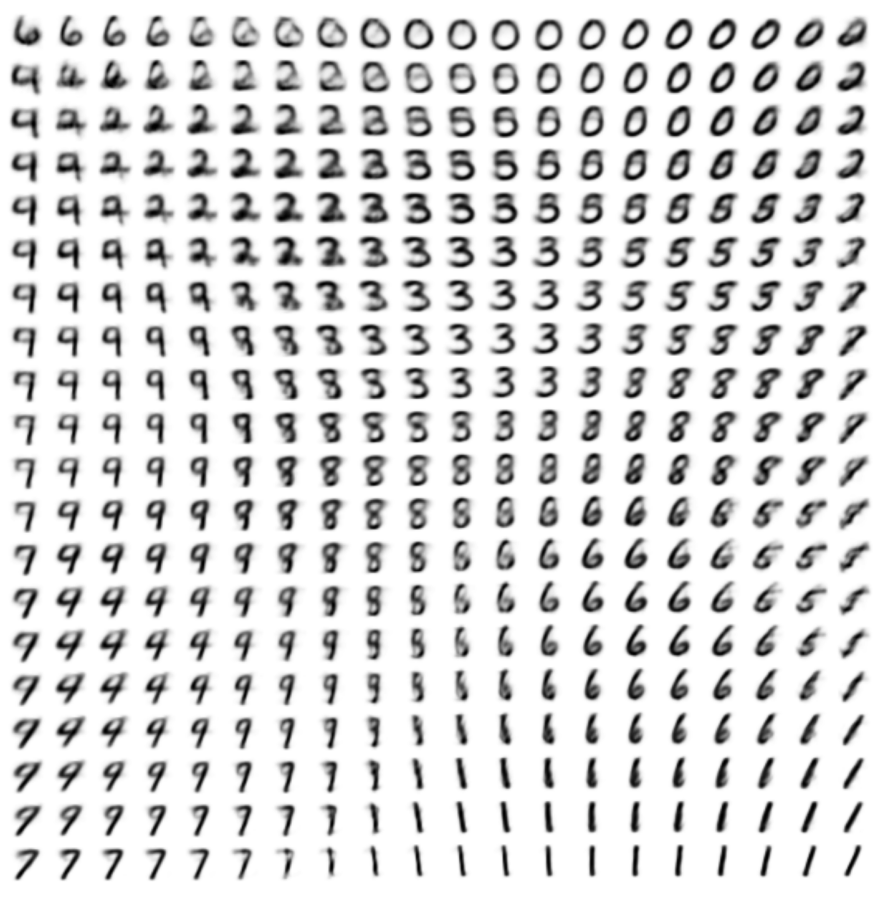
Interpolating over MNIST digits by interpolating over latent variables The VAE can be applied to images $x$ in order to learn interesting latent representations. The VAE paper contains a few examples on the Frey face dataset on the MNIST digits. On the face dataset, we can interpolate between facial expressions by interpolating between latent variables (e.g. we can generate smooth transitions between “angry” and “surprised”). On the MNIST dataset, we can similarly interpolate between numbers.

The authors also compare their methods against three alternative approaches: the wake-sleep algorithm, Monte-Carlo EM, and hybrid Monte-Carlo. The latter two methods are sampling-based approaches; they are quite accurate, but don’t scale well to large datasets. Wake-sleep is a variational inference algorithm that scales much better; however it does not use the exact gradient of the ELBO (it uses an approximation), and hence it is not as accurate as AEVB. The paper illustrates this by plotting learning curves.