Map inference
This section will explore in more detail the problem of MAP inference in graphical models. Recall that MAP inference in a graphical model corresponds to the following optimization problem:
In the previous section, we briefly showed how to solve this problem within the same message passing framework as marginal inference. We will now look at more efficient specialized methods.
The challenges of MAP inference
In a way, MAP inference is easier than marginal inference. One reason for this is that the intractable partition constant does not depend on and can be ignored:
Marginal inference can also be seen as computing and summing all assignments to the model, one of which is the MAP assignment. If we replace summation with maximization, we can also find the assignment with the highest probability; however, there exist more efficient methods that this sort of enumeration-based approach.
Note, however, that MAP inference is still not an easy problem in the general case. The above optimization objective includes many intractable problems as special cases, e.g. 3-sat. We may reduce 3-sat to MAP inference by constructing for each clause a factor that equals one if satisfy clause , and otherwise. Then, the 3-sat instance is satisfiable if and only if the value of the MAP assignment equals the number of clausesWe may also use a similar construction to prove that marginal inference is NP-hard. The high-level idea is to add an additional variable that equals when all the clauses are satisfied, and zero otherwise. Its marginal probability will be greater than zero iff the 3-sat instance is satisfiable. .
Nonetheless, we will see that the MAP problem is easier than general inference, in the sense that there are some models in which MAP inference can be solved in polynomial time, while general inference is NP-hard.
Examples
Many interesting examples of MAP inference are instances of structured prediction, which involves doing inference in a conditional random field (CRF) model :
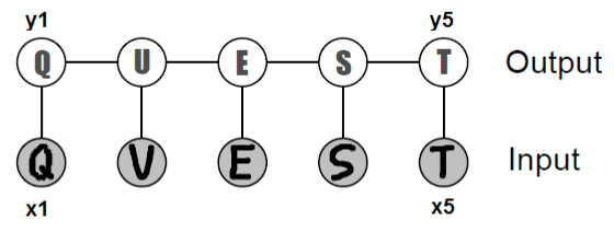
Chain-structured conditional random field for optical character recognition.
We discussed structured prediction in detail when we covered CRFs.
Recall that our main example was handwriting recognition, in which we are given
images of characters in the form of pixel matrices; MAP inference in this setting amounts to jointly recognizing the most likely word encoded by the images.
Another example of MAP inference is image segmentation; here, we are interested in locating an entity in an image and label all its pixels. Our input is a matrix of image pixels, and our task is to predict the label , indicating whether each pixel encodes the object we want to recover. Intuitively, neighboring pixels should have similar values in , i.e. pixels associated with the horse should form one continuous blob (rather than white noise).
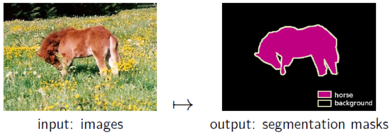
An illustration of the image segmentation problem.
This prior knowledge can be naturally modeled in the language of graphical models via a Potts model. As in our first example, we can introduce potentials that encode the likelihood that any given pixel is from our subject. We then augment them with pairwise potentials for neighboring , which will encourage adjacent ’s to have the same value with higher probability.
Graphcuts
We will start our discussion with an efficient exact MAP inference algorithm for certain Potts models. Unlike previously-seen methods (e.g. the junction tree algorithm), this algorithm will be tractable even when the model will have large treewidth.
Suppose we are given a binary pairwise MRF in which edge energies (i.e. log-edge factors) have the form
where is a cost that penalizes edge mismatches. Assume also that nodes have unary potentials; we can always normalize the nodes’ energies so that or and .
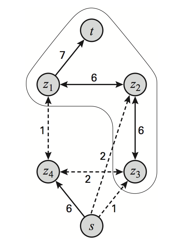
Formulating the segmentation task in a 2x2 MRF as a graph cut problem. Dashed edges are part of the min-cut. (Source: Machine Learning: A Probabilistic Perspective).
The motivation for this model comes from image segmentation. We are looking for an assignment that minimizes the energy, which (among other things) tries to reduce discordance between adjacent variables.
We can formulate energy minimization in this type of model as a min-cut problem in an augmented graph : we construct by adding special source and sink nodes to our PGM graph; the node is connected to nodes with by an edge with weight ; the node is connected to nodes with by an edge with weight . Finally, all the edges of the original graph get as their weight.
It is not hard to see that by construction, the cost of a min-cut in this graph will equal the minimum energy in the model. In particular, all nodes on the side of the cut receive an assignment of , and all the ones that are on the side receive an assignment of one. The edges between the nodes that disagree are precisely the ones that are in the min-cut.
The fastest algorithms for computing min-cuts in a graph take or time. Similar techniques can also be applied in slightly more general types of models with a certain type of edge potentials that are called submodular. We refer the reader to a textbook (e.g. Koller and Friedman) for more details.
Linear programming-based approaches
Although graphcut-based methods recover the exact MAP assignment, they are only applicable in certain restricted classes of MRFs. The algorithms we will see next solve the MAP problem approximately, but can applied in much larger classes of graphical models.
Linear programming
Our first approximate inference strategy consists in reducing MAP inference to integer linear programming. Linear programming (LP) — also known as linear optimization — refers to a class of problems of the form
where , and , are problem parameters.
Problems of this form are found in almost every field of science and engineering. They have been extensively studied since the 30’s, which has led to both an extensive theoryA major breakthrough of applied mathematics in the 80’s was the development polynomial-time algorithms for linear programming. , as well as practical tools that can solve very large LP instances (100,000 variables or more) in a reasonable time.
Integer linear programming (ILP) is an extension of linear programming in which we also require that . Unfortunately, this makes optimization considerably more difficult, and ILP is in general NP-hard. Nonetheless, there are many heuristics for solving ILP problems in practice, and commercial solvers can handle instances with thousands of variables or more.
One of the main techniques for solving ILP problems is rounding. The idea of rounding is to relax the requirement that into , solve the resulting LP, and then round the LP solution to its nearest integer value. This approach works surprisingly well in practice and has theoretical guarantees for some classes of ILPs.
Formulating MAP inference as ILP
For simplicity, let’s look at MAP in pairwise MRFs. We can reduce the MAP objective to integer linear programming by introducing two types of indicator variables:
- A variable for each and state .
- A variable for each edge and pair of states .
We can rewrite the MAP objective in terms of these variables as
We would like to optimize over these ’s; for that we also need to introduce constrains. First, we need to force each cluster to choose a local assignment:
These assignments must also be consistent:
Together, these constraints along with the MAP objective yield an integer linear program, whose solution equals the MAP assignment. This ILP is still NP-hard, but we have an easy way to transform this into an (easy to solve) LP via relaxation. This is the essence of the linear programming approach to MAP inference.
In general, this method will only give approximate solution. An important special case are tree-structured graphs, in which the relaxation is guaranteed to always return integer solution, which are in turn optimalSee e.g. the textbook of Koller and Friedman for a proof and a more detailed discussion. .
Dual decomposition
Let us now look at another way to transform the MAP objective into a more amenable optimization problem. Suppose that we are dealing with an MRF of the form
where denote arbitrary factors (e.g. the edge potentials in a pairwise MRF)These short notes are roughly based on the tutorial by Sontag et al., to which we refer the reader for a full discussion. . Let us use to denote the optimal value of this objective and let denote the optimal assignment.
The above objective is difficult to optimize because the potentials are coupled. Consider for a moment an alternative objective where we optimize the potentials separately:
This would be easy optimize, but would only give us an upper bound on the value of the true MAP assignment. To make our relexation tight, we would need to introduce constraints that encourage consistency between the potentials:
The dual decomposition approach consists in softening these constraints in order to achieve a middle ground between the two optimization objective defined above.
We will achieve this by first forming the Lagrangian for the constrained problem, which is
The variables are called Lagrange multipliers; each of them is associated with a constraintThere is a very deep and powerful theory of constrained optimization centered around Lagrangians. We refer the reader to a course on convex optimization for a thorough discussion. . Observe that is a valid assignment to the Lagrangian; its value equals for any , since the Lagrange multipliers are simply multiplied by zero. This shows that the Lagrangian is an upper bound on :
In order to get the tightest such bound, we may optimize over . It turns out that by the theory of Lagarange duality, at the optimal , this bound will be exactly tight, i.e.
It is actually not hard to prove this in our particular setting. To see that, note that we can reparametrize the Lagrangian as:
Suppose we can find dual variables such that the local maximizers of and agree; in other words, we can find a such that and . Then we have that
The first equality follows by definition of , while the second follows holds because terms involving Lagrange multipliers cancel out when and agree.
On the other hand, we have by the definition of that
which implies that .
This argument has shown two things:
- The bound given by the Lagrangian can be made tight for the right choice of .
- To compute , it suffices to find a at which the local sub-problems agree with each other. This happens surprisingly often in practice.
Minimizing the objective
There exist several ways of computing , of which we will give a brief overview.
Since the objective is continuous and convexThe objective is a pointwise max of a set of affine functions. , we may minimize it using subgradient descent. Let and let . It can be shown that the gradient of w.r.t. equals if and zero otherwise; similarly, equals if and zero otherwise. This expression has the effect of decreasing and increasing , thus bringing them closer to each other.
To compute these gradients we need to perform the operations and . This is possible if the scope of the factors is small, if the graph has small tree width, if the factors are constant on most of their domain, and in many other useful special cases.
An alternative way of minimizing is via block coordinate descent. A typical way of forming blocks is to consider all the variables associated with a fixed factor . This results in updates that are very similar to loopy max-product belief propagation. In practice, this method may be faster than subgradient descent, is guaranteed to decrease the objective at every step, and does not require tuning a step-size parameter. Its drawback is that it does not find the global minimum (since the objective is not strongly convex).
Recovering the MAP assignment
As we have seen above, if a solution agrees on the factors for some , then we can guarantee that this solution is optimal.
If the optimal do not agree, finding the MAP assignment from this solution is still NP-hard. However, this is usually not a big problem in practice. From the point of view of theoretical guarantees, if each has a unique maximum, then the problem will be decodable. If this guarantee is not met by all variables, we can clamp the ones that can be uniquely decoded to their optimal values and use exact inference to find the remaining variables’ values.
Other methods
Local search
A more heuristic-type solution consists in starting with an arbitrary assignment and perform “moves” on the joint assignment that locally increase the probability. This technique has no guarantees; however, we can often use prior knowledge to come up with highly effective moves. Therefore, in practice, local search may perform extremely well.
Branch and bound
Alternatively, one may perform exhaustive search over space of assignments, while pruning branches that can be provably shown not to contain a MAP assignment. The LP relaxation or its dual to obtain upper bounds useful for pruning trees.
Simulated annealing
A third approach is to use sampling methods (e.g. Metropolis-Hastings) to sample from . The parameter is called the temperature. When , is close to the uniform distribution, which is easy to sample form. As , places more weight on , the quantity we want to recover. However, since this distribution is highly peaked, it is also very difficult to sample from it.
The idea of simulated annealing is to run a sampling algorithm starting with a high , and gradually decrease it, as the algorithm is being run. If the “cooling rate” is sufficiently slow, we are guaranteed to eventually find the mode of our distribution. In practice, however, choosing the rate requires a lot of tuning. This makes simulated annealing somewhat difficult to use in practice.